What is PyGran?¶

PyGran is an object-oriented library written primarily in Python for Discrete Element Method (DEM) simulation and analysis. The main purpose of PyGran is to provide an easy and intuitive way for performing technical computing in DEM, enabling flexibility in how users interact with data from the onset of a simulation and until the post-processing stage. In addition to providing a brief tutorial on installing PyGran for Unix systems, this manual focuses on 2 core modules (Fig. 1) in PyGran : simulation which provides engines for running DEM simulation and enables analysis of contact mechanical models, and analysis which contains methods and submodules for processing DEM data. PyGran is released under the GNU General Public License (GPL v2.0), and its code base is available from github.

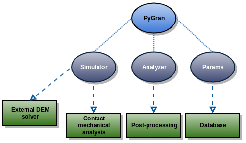
PyGran modules — Fig. 1 A diagram that shows the hierarchical structure of *PyGran* in terms of its core modules that can be imported from a Python script.¶

Brief summary of DEM¶

The Discrete Element Method (DEM) is the application of Newtonian mechanics to a set of interacting particles that are usually assumed to be spherical in shape. For a spherical particle \(i\) that undergoes translation and rotation and of moment of inertia \(I_i\) and volume \(V_i\), its dynamical equations are

(1)¶\[ \begin{align}\begin{aligned}\rho V_i a_i &= \sum_j F_{ij} + F_{b_i},\\I_i \alpha_i &= \sum_j T_{ij}.\end{aligned}\end{align} \]

The true mass density of the particles is \(\rho\), \(F_{ij}\) is the surface contact force between particle \(i\) and its neighbors (summed over \(j\)), \(F_{b_i}\) is a body force acting on particle \(i\) (such as gravity, i.e. \(F_{b_i} = \rho V_i g\)), and \(T_{ij}\) is the torque between particle \(i\) and its neighbors that is limited by the static friction coefficient \(\mu\).

DEM simulation involves the numerical solution of Eqs. (1) by decomposing the space the particles occupy into a grid of connected nearest-neighbor lists that enable fast and efficient computation of inter-particle surface forces. For every discrete timestep, all forces acting on each particle are computed, and the particle positions are updated based on the discretized form of Eqs. (1).

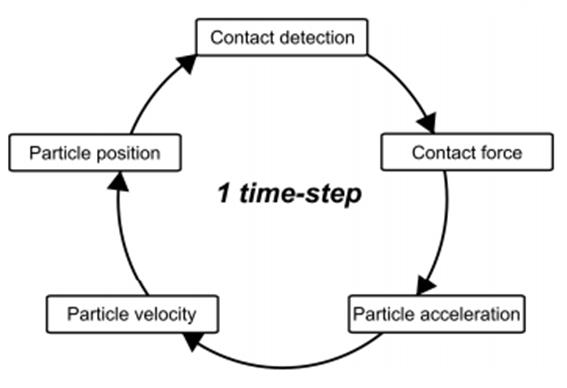
DEM cycle — Fig. 2 A flowchart that shows the different stages involved in completing a single DEM timestep.¶

The form of the surface contact forces depends on the type of the bodies interacting with each other. Visco-elastic particles for instance can be modeled as two connected spring-dashpots. More sophisticated models assume particles behave as elasto-plastic spheres that undergo plastic deformation when the pressure exceeds a yield stress characteristic of the material the particles are composed of. Irrespective of the method energy dissipation is modeled, DEM usually assumes the two spherical particles in contact experience an elastic repulsive force that follows Hertz’ law. In addition to dissipation, the particles can experience an attractive cohesive force depending on their size. The contact models implemented in PyGran are discussed in the Simulation pat. For a comprehensive review of DEM and contact mechanics, see [PoschelS05].

As of version 1.1, PyGran supports non-spherical particle simulation with the multisphere method (MS-DEM) [KERWS08]. In this method, non-spherical particles are approximated by a series of spheres glued together as shown in Fig. 3.

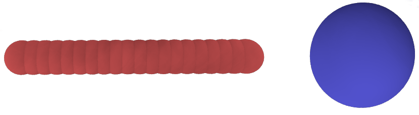
Multisphere particle — Fig. 3 In DEM, particles are usually represented as spheres (right); non-spherical particles (such as a rod, left) can be approximated with a group of glued spheres¶

Installation¶

Quick installation with PyPi¶

The easiest way to install the latest stable version of PyGran is with PyPi:

pip install pygran --user

This will install pygran_analysis and pygran_sim packages. If you’re interested in running only analysis or simulation, then you should install whichever package you require.

Configuration with LIGGGHTS¶

PyGran has been tested with LIGGGHTS-PUBLIC versions 3.4, 3.7, and 3.8. For running DEM simulation with LIGGGHTS, the latter must be compiled as a shared library (shared object on Unix/Linux systems), which PyGran will attempt to find. By default, PyGran searches for any available installation of libliggghts.so and writes its path name to the 1st line in ~/.config/PyGran/liggghts.ini. PyGran will also attempt to find the LIGGGHTS version and source path, and write each to the 2nd and 3rd lines, respectively, in the .ini file. Alternatively, in case multiple versions are installed on the system or if the library filename is not libliggghts.so, users can specify the name of the shared object and optionally its source code path and version via:

import PyGran

PyGran.configure(
    path='/home/user/.local/lib/custom_libliggghts.so',
    version='3.8.0',
    src='/path/to/LIGGGHTS-3.8.0/src'
)

This produces a ~/.config/PyGran/liggghts.ini file for LIGGGHTS v3.8 shown below:

library=/home/user/.local/lib/custom_libliggghts.so
src=/path/to/LIGGGHTS-3.8.0/src
version=3.8.0

If config.ini file is not found, PyGran will create one.

Compiling LIGGGHTS¶

PyGran’s setup enables the compilation of LIGGGHTS-PUBLIC from its source code available from the CFDEM github repository via:

python setup.py build_liggghts

The command above will clone the LIGGGHTS-PUBLIC repository and compile the code as a shared library (libliggghts.so) in LIGGGHTS-PUBLIC/src. This requires git, gcc, and an MPI installation available on the system.

Installation example: ubuntu 18.04 (LTS)¶

The section below covers a fresh local installation of PyGran & LIGGGHTS form source code. They have been tested with python 3, gcc v7.x, and LIGGGHTS v3.8. For global installs, remove --user from the commands and use sudo instead.

First, fire up a terminal in order to update the system and install all dependencies via:

sudo apt-get update && sudo apt-get install gcc libopenmpi-dev python3-setuptools python3-pip ipython3 git python3-matplotlib libvtk6-dev -y

Let’s now clone the PyGran source code:

git clone https://github.com/anabiman/pygran.git
cd pygran

Install PyGran dependencies with pip:

pip3 install .[extra]

If LIGGGHTS is not available as a shared library, run:

python3 setup.py build_liggghts

This will clone the LIGGGHTS-PUBLIC repository and compile the code as a shared object. The process takes a few minutes to finish. Once this is done, we can finally install PyGran:

pip3 install .

Testing PyGran¶

In order to test PyGran, we need to install pytest (pip install pytest does the trick). Now let’s run a simple flow problem in order to make sure everything works fine. Open a terminal and run from the source dir:

pytest -v pygran/tests/test_sim

The process should take about 1-5 mins to finish, depending on the core clock cycle. If successful, this command should create an output directory (‘DEM_flow’) which contains the trajectory and restart files stored in ‘traj’ and ‘restart’ directories, respectively.

In order to test the analysis module, run from the source dir:

pytest -v pygran/tests/test_analysis --trajf "DEM_flow/traj/particles*.dump"

The process should take few seconds to execute. If no exception is raised, then you know you can safely run PyGran for both simulation and analysis.